I’ve been working with Bobby from Pewlett Hackard to analyze employee data, breaking down employee names, departments, titles, and tenure. Bobby’s manager has given both of you two more assignments: determine the number of retiring employees per title, and identify employees who are eligible to participate in a mentorship program. I have provided a written report that summarizes the analysis to help prepare Bobby’s manager for the “silver tsunami” as many current employees reach retirement age.
For this analysis I had to use Database Keys to establish the relationship between multiple tables, for this I focused on the Primary and Foreign Keys.
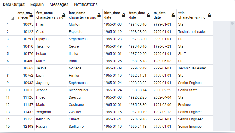
I used an ERD (Entity Relationship Diagram) to help with highlighting the relationships between each of the tables. Once each of the tables were joined together, I was then able to create the tables needed to help show the retiring employees by title and identify the employees eligible to participate in the mentorship program.
Results of Data
Deliverable 1: The Number of Retiring Employees by Title
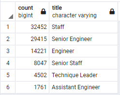
These results show that 133,776 employees that could retire and also provides their title.
See the breakdown by title below:
32,452 Staff
29,415 Senior Engineer
14,221 Engineer
8,047 Senior Staff
4,502 Technique Leader
1,761 Assistant Engineer
Deliverable 2: The Employees Eligible for the Mentorship Program
There were a total of 1,940 employees eligible for the mentorship program.
Summary
After analyzing the data to provide for Bobby to present to his managers, I believe this information will help with forcasting how many retirees to prepare for. They will also be able to predict and plan a hiring campaign from this data to fill the turnover from retirements.
PLEASE NOTE: This is beta software and may not work as intended. Please file issues if you find something broken!
This is a new release of software. It will have bugs.
I mostly mine ETH, so mining other coins may or may not cause problems. Report any you find, please.
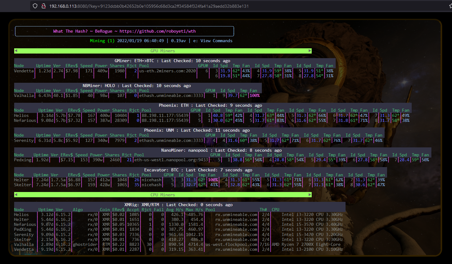
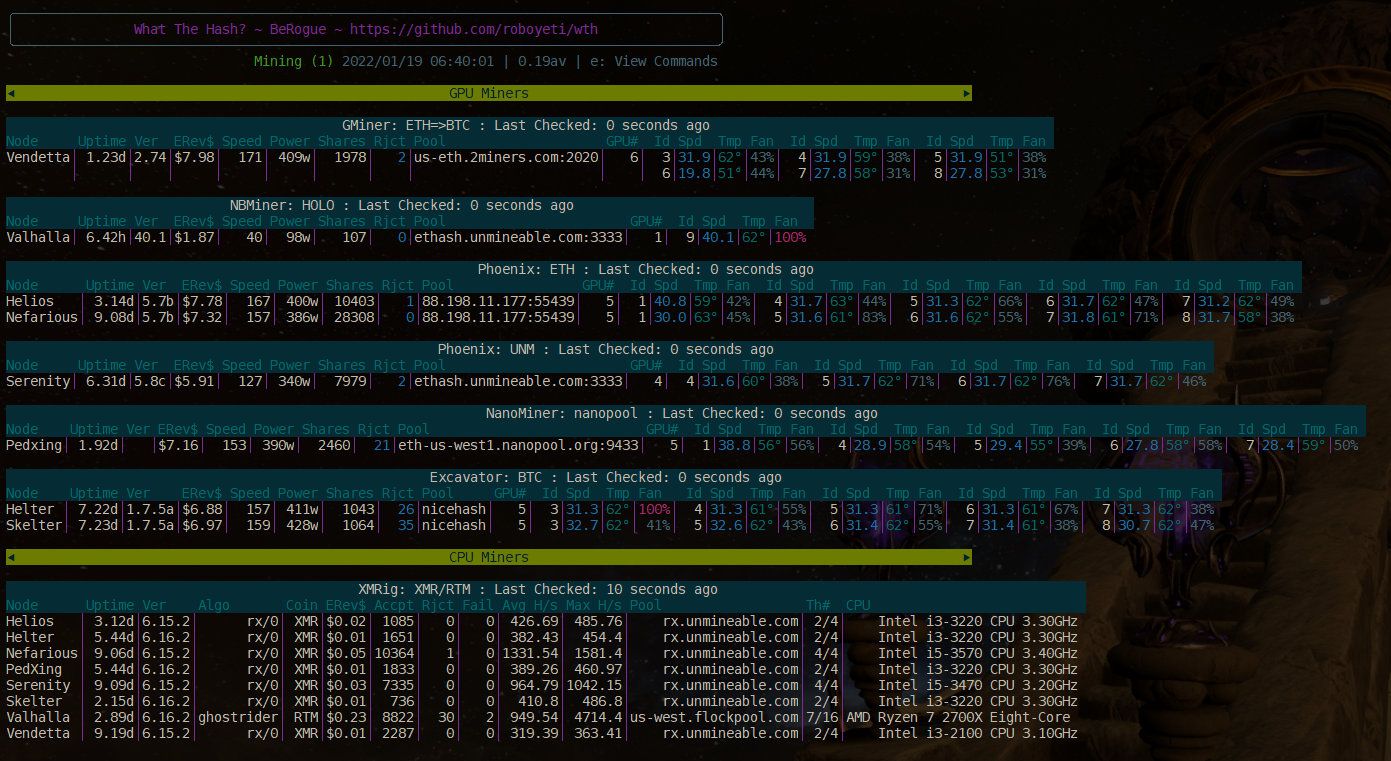
What is “What the Hash?”?
WTH is a “consolidator”, that gathers data from different APIs, such as those on miners and pools, to bring it
all together into one interface (console, web, and/or API).
WTH was designed with the goal of providing an expandable, quick
health status / earnings viewer for cryptocurrency related interests, miners, etc.
It was originally developed to allow me to get a fast view on the health of all my GPU/CPU miners, regardless of
miner software or pool software. Mostly, I was frustrated at looking at half a dozen or more web pages just to check in on miners, pools, and portfolios.
It isn’t meant to compete with fancy web UIs with charts and graphs (yet), but can easily run alongside those. I have found that I rely less and less on the remote pool web interfaces to give me updates in addition to things like the portfolio not requiring me to share my holdings with external websites.
With very little interaction, you should be able to see the basics of your cryptocurrency
world. Adding more mining pools, staking & liquidity pools, crypto portfolios, and more
is the plan.
WTH also offers an API for other systems to use the collected data. The primary
goal of this is so we can offer a more advanced Web UI in the future, but it also tries
to serve as a single API protocol for many different miners and pools out in the wild.
You can help us and add your own modules as well! The coding required can be fairly
simplistic, depending on the remote API, and help from us can get
your module added quickly. Don’t program? You can request the new module, but those who
donate get the most attention (see donation addresses below). Requests can go here:
Ideas
WTH should be considered beta software. I wrote it as a quick tool for myself, then it
proved so helpful, I started to grow it, and then I decided to release it. Contributions
to the code base are welcome, but only do so if you understand that this software is beta and
things will change.
With either web interface (basic or API), you can enable a private key to restrict access
Enable in config and set your key
Add &key=<your_key> to the URL for both interfaces to send it with request.
Other stuff
wthlab.rb is an interactive shell with a WTH application spun up with your config.
wthd.rb is an untested daemonized wth for OSs that support fork.
Use: ruby ./wthd.rb [start|stop|status|restart]
To detach from console, you can also set config option “console_out” to false
When a URL is visible on the console, you may be able to CTRL + Mouse click it to open in browser. Terminal and OS mileage may vary.
Configuration
The default config file is “wth_config.yml”
Example config file is “wth_config_example.yml”
You can run with different config file using arguments to wth: -c or –config
Example: ruby wth.rb -c wth_my_other_config.yml
Configuration – Modules
Modules are interfaces to software installed on your mining machines or remote APIs. You may have to install software yourself on one or more machines to get the features of a module.
Specific configuration options can be found in the example config.
Brief documentation for how to enable APIs for a specific module target can be found in docs/modules/<target_name>.
List of supported modules and the config “api” entry for them:
GPU Miners
Excavator (Nicehash Nvidia Miner) = “nice_hash”
Claymore Miner = “claymore” (untested)
Phoenix Miner = “phoenix”
T-Rex Miner = “t_rex_unm”
GMiner = “g_miner”
LolMiner = “lol_miner”
NanoMiner = “nano_miner”
NBMiner = “nbminer”
CPU Miners
XMRig = “xmrig”
Cpuminer-gr = “raptoreum”
Cpuminer- = “cpuminer” (Untested other than cpuminer-gr)
Harddrive Miners
Signum Miner (via pool API) = “signum_pool_miner”
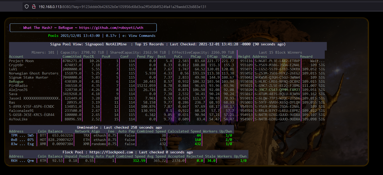
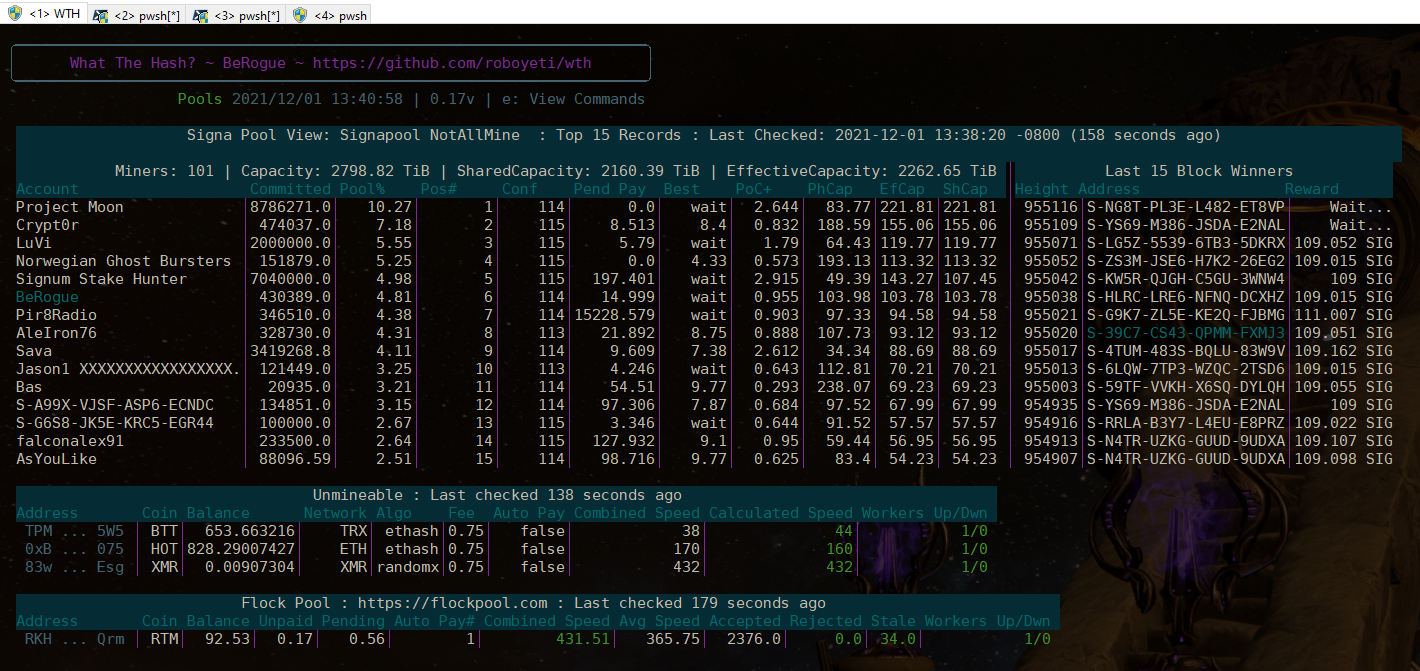
Pools
2Miners = “2miners_pool”
Nano Pool = “nano_pool”
Signum Pool API = “signum_pool_view”
Flock Pool (RTM) = “flock_pool”
Unmineable (Address API) = “unmineable” (best with local Tor installation for socks poxying)
Tokens
Signum Tokens = “signum_tokens”
ZapperFi = “zapper_fi” – Includes ETH tokens, Avalanche, and more. See http://zapper.fi
Portfolio
Coingecko = “coin_gecko” – Build your own personal portfolio without sharing your data. Pricing is possible on any coin CoinGecko supports. See http://coingecko.com
Hardware
LibreHardwareMonitor +WMI GPU/CPU monitoring on Win32 = “ohm_gpu_w32” (Experimental)
— Comaptibility with OpenHardwareMonitor possible, but untested. (Experimental)
web_server_start: [true|false] = Run web server or not
default_module_frequency: [integer] = Number of seconds between default module check. Override per module with “every:” directive. Some modules have minimums enforced to ensure you don’t get yourself banned or overload remote APIs that are generously provided by others for free.
Configuration – Web Server
The following web server config options are:
web_server:
html_out: [true|false] = Enable the console => html conversion. Turning this off will leave the API running, if that is enabled. True default.
port: [integer] = Port number to run basic and API on. Default is 8080
host: [network_addr] = For local machine access, set to 127.0.0.1 or localhost, 0.0.0.0 for all interfaces (default), or specific IP address for a specific interface.
ssl: [true|false] = Enables SSL. Your SSL cert and pkey pem files will be generated for you and stored in “data/ssl/*.pem”. You can replace those with your own if you desire.
api: [true|false] = Enable the API interface for the web server. Default false.
key: [string] = User chosen string to act as you private web access string. Append all URL requests with &api_key=<your_key> if you set this.
Configuration – Misc Notes
Tor SOCKS and Http Proxy is available, but currently is enabled per module with no global mechanism to set it yet and not all modules support it (those who use custom network code: claymore, phoenix, cpuminer, zapper.fi).
Donate!
Donations are very welcome and if you find this program helpful. If you want a
miner, pool, or other crypto currency related site/tool integrated, donations also go a
long way to convince me to investigate if it is possible and spend the personal time
adding something I don’t need myself.
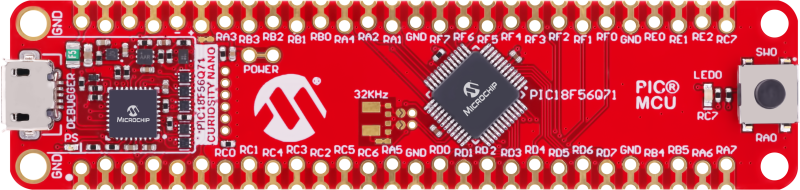
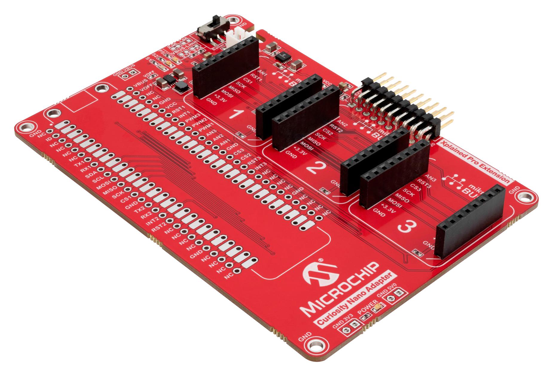
Analog-to-Digital Converter with Computation (ADCC) and Context Switching — Context Switching Using PIC18F56Q71 Microcontroller with MCC Melody
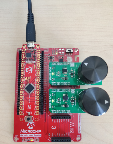
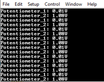
This code example demonstrates how to perform two Analog-to-Digital Converter with Computation (ADCC) and Context Switching conversions from two input channels that have different peripheral configurations by using the Context Switching feature. The ADCC with Context Switching supports up to four configuration contexts and offers the option of switching between these contexts at runtime. By using this feature, a single ADCC with Context Switching peripheral is used to capture data from multiple analog input channels, each one of them having its own configuration. The conversion results are processed and displayed on a terminal software by using serial communication via an UART peripheral.
Related Documentation
More details and code examples on the PIC18F56Q71 can be found at the following links:
This example shows how to configure the ADCC with Context Switching using the MPLAB® Code Configurator. Also, it demonstrates the use of context switching for acquiring data from multiple analog inputs.
This chapter demonstrates how to use the MPLAB® X IDE to program an PIC® device with an Example_Project.X. This can be applied to any other project.
Connect the board to the PC.
Open the Example_Project.X project in MPLAB® X IDE.
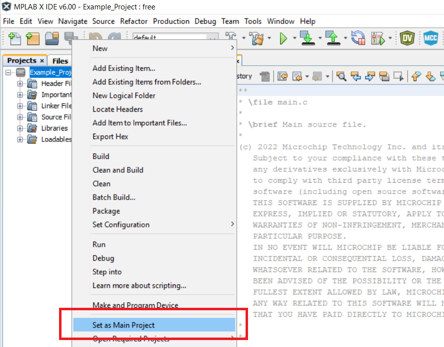
Set the Example_Project.X project as main project.
Right click the project in the Projects tab and click Set as Main Project.
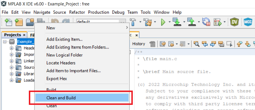
Clean and build the Example_Project.X project.
Right click the Example_Project.X project and select Clean and Build.
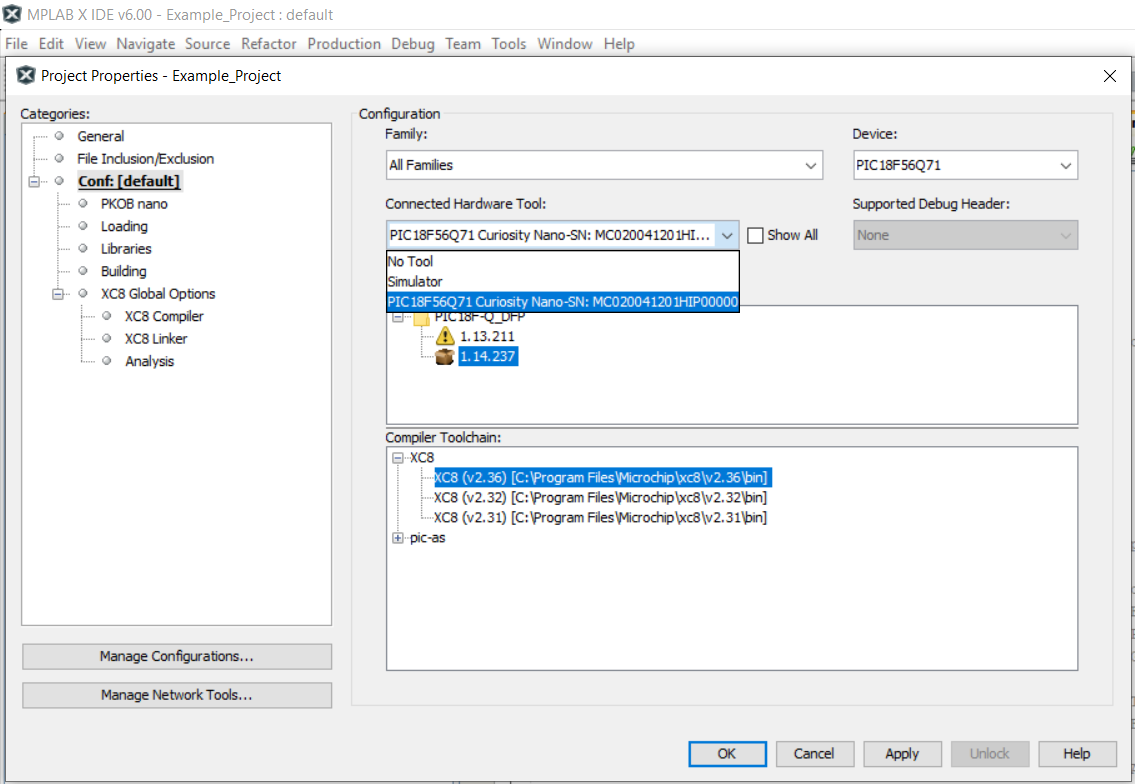
Select PICxxxxx Curiosity Nano in the Connected Hardware Tool section of the project settings:
Right click the project and click Properties.
Click the arrow under the Connected Hardware Tool.
Select PICxxxxx Curiosity Nano (click the SN), click Apply and then click OK.
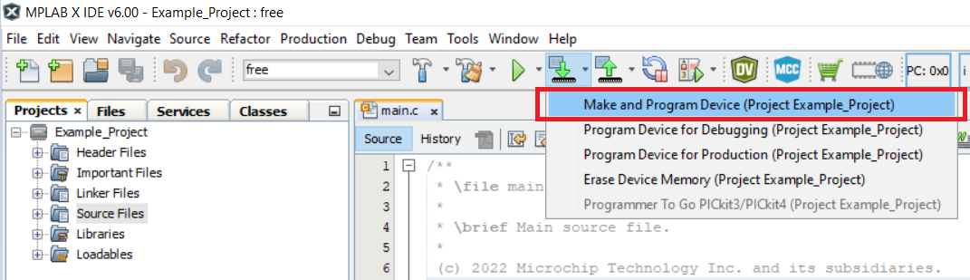
Program the project to the board.
Right click the project and click Make and Program Device.
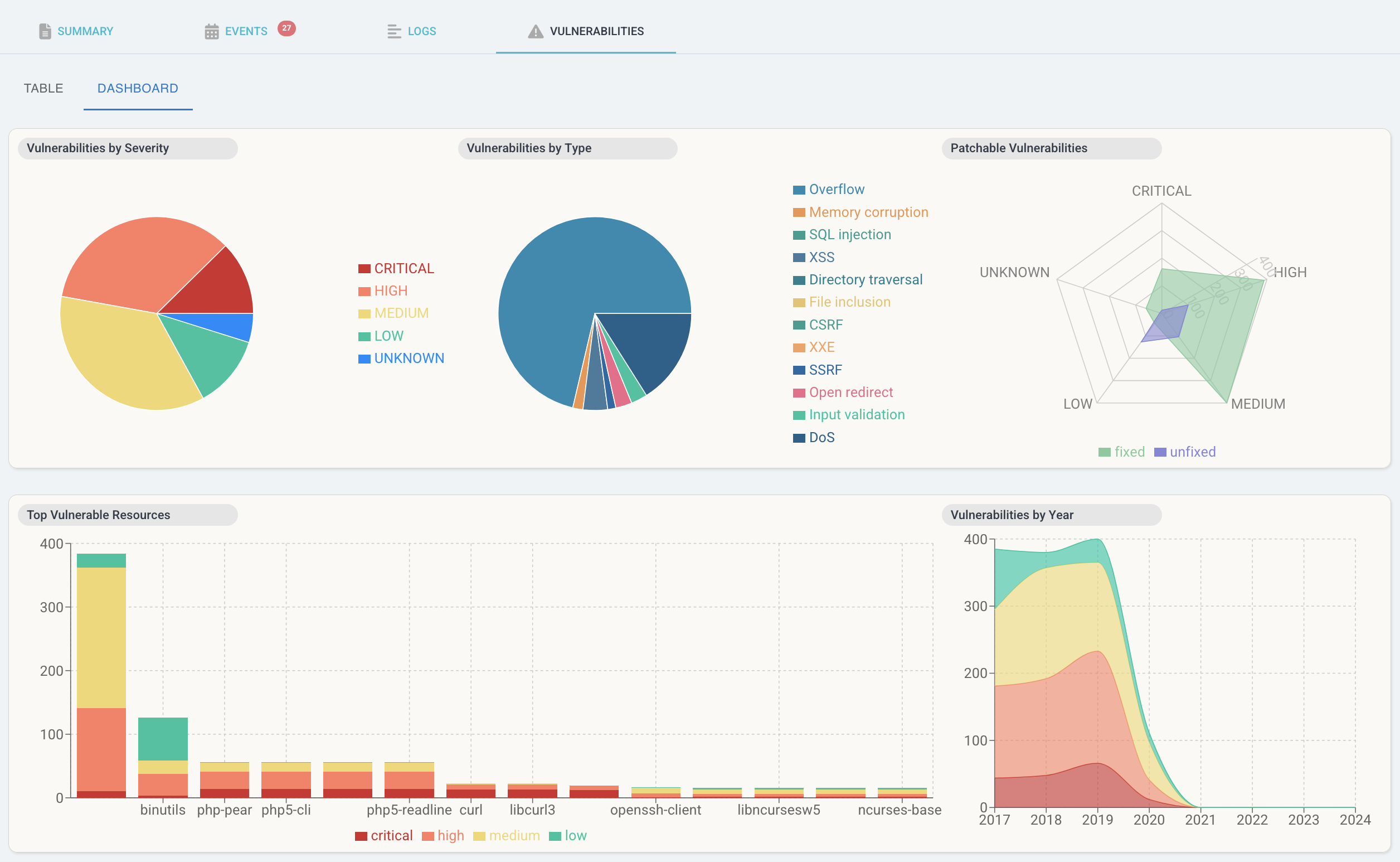
Argo CD UI extension that displays vulnerability report data from Trivy, an open source security scanner.
Trivy creates a vulnerability report Kubernetes resource with the results of a security scan. The UI extension then parses the report data and displays it as a grid and dashboard viewable in Pod resources within the Argo CD UI.
The UI extension needs to be installed by mounting the React component in Argo CD API server. This process can be automated by using the argocd-extension-installer. This installation method will run an init container that will download, extract and place the file in the correct location.
Helm
To install the UI extension with the Argo CD Helm chart add the following to the values file:
server:
extensions:
enabled: trueextensionList:
- name: extension-trivyenv:
# URLs used in example are for the latest release, replace with the desired version if needed
- name: EXTENSION_URLvalue: https://github.com/mziyabo/argocd-trivy-extension/releases/latest/download/extension-trivy.tar
- name: EXTENSION_CHECKSUM_URLvalue: https://github.com/mziyabo/argocd-trivy-extension/releases/latest/download/extension-trivy_checksums.txt
Kustomize
Alternatively, the yaml file below can be used as an example of how to define a kustomize patch to install this UI extension:
apiVersion: apps/v1kind: Deploymentmetadata:
name: argocd-serverspec:
template:
spec:
initContainers:
- name: extension-trivyimage: quay.io/argoprojlabs/argocd-extension-installer:v0.0.1env:
# URLs used in example are for the latest release, replace with the desired version if needed
- name: EXTENSION_URLvalue: https://github.com/mziyabo/argocd-trivy-extension/releases/latest/download/extension-trivy.tar
- name: EXTENSION_CHECKSUM_URLvalue: https://github.com/mziyabo/argocd-trivy-extension/releases/latest/download/extension-trivy_checksums.txtvolumeMounts:
- name: extensionsmountPath: /tmp/extensions/securityContext:
runAsUser: 1000allowPrivilegeEscalation: falsecontainers:
- name: argocd-servervolumeMounts:
- name: extensionsmountPath: /tmp/extensions/volumes:
- name: extensionsemptyDir: {}
Implementation of iTransformer – SOTA Time Series Forecasting using Attention networks, out of Tsinghua / Ant group
All that remains is tabular data (xgboost still champion here) before one can truly declare “Attention is all you need”
In before Apple gets the authors to change the name.
The official implementation has been released here!
Appreciation
StabilityAI and 🤗 Huggingface for the generous sponsorship, as well as my other sponsors, for affording me the independence to open source current artificial intelligence techniques.
Greg DeVos for sharing experiments he ran on iTransformer and some of the improvised variants
Install
$ pip install iTransformer
Usage
importtorchfromiTransformerimportiTransformer# using solar energy settingsmodel=iTransformer(
num_variates=137,
lookback_len=96, # or the lookback length in the paperdim=256, # model dimensionsdepth=6, # depthheads=8, # attention headsdim_head=64, # head dimensionpred_length= (12, 24, 36, 48), # can be one prediction, or manynum_tokens_per_variate=1, # experimental setting that projects each variate to more than one token. the idea is that the network can learn to divide up into time tokens for more granular attention across time. thanks to flash attention, you should be able to accommodate long sequence lengths just fineuse_reversible_instance_norm=True# use reversible instance normalization, proposed here https://openreview.net/forum?id=cGDAkQo1C0p . may be redundant given the layernorms within iTransformer (and whatever else attention learns emergently on the first layer, prior to the first layernorm). if i come across some time, i'll gather up all the statistics across variates, project them, and condition the transformer a bit further. that makes more sense
)
time_series=torch.randn(2, 96, 137) # (batch, lookback len, variates)preds=model(time_series)
# preds -> Dict[int, Tensor[batch, pred_length, variate]]# -> (12: (2, 12, 137), 24: (2, 24, 137), 36: (2, 36, 137), 48: (2, 48, 137))
For an improvised version that does granular attention across time tokens (as well as the original per-variate tokens), just import iTransformer2D and set the additional num_time_tokens
Update: It works! Thanks goes out to Greg DeVos for running the experiment here!
Update 2: Got an email. Yes you are free to write a paper on this, if the architecture holds up for your problem. I have no skin in the game
importtorchfromiTransformerimportiTransformer2D# using solar energy settingsmodel=iTransformer2D(
num_variates=137,
num_time_tokens=16, # number of time tokens (patch size will be (look back length // num_time_tokens))lookback_len=96, # the lookback length in the paperdim=256, # model dimensionsdepth=6, # depthheads=8, # attention headsdim_head=64, # head dimensionpred_length= (12, 24, 36, 48), # can be one prediction, or manyuse_reversible_instance_norm=True# use reversible instance normalization
)
time_series=torch.randn(2, 96, 137) # (batch, lookback len, variates)preds=model(time_series)
# preds -> Dict[int, Tensor[batch, pred_length, variate]]# -> (12: (2, 12, 137), 24: (2, 24, 137), 36: (2, 36, 137), 48: (2, 48, 137))
Experimental
iTransformer with fourier tokens
A iTransformer but also with fourier tokens (FFT of time series is projected into tokens of their own and attended along side with the variate tokens, spliced out at the end)
importtorchfromiTransformerimportiTransformerFFT# using solar energy settingsmodel=iTransformerFFT(
num_variates=137,
lookback_len=96, # or the lookback length in the paperdim=256, # model dimensionsdepth=6, # depthheads=8, # attention headsdim_head=64, # head dimensionpred_length= (12, 24, 36, 48), # can be one prediction, or manynum_tokens_per_variate=1, # experimental setting that projects each variate to more than one token. the idea is that the network can learn to divide up into time tokens for more granular attention across time. thanks to flash attention, you should be able to accommodate long sequence lengths just fineuse_reversible_instance_norm=True# use reversible instance normalization, proposed here https://openreview.net/forum?id=cGDAkQo1C0p . may be redundant given the layernorms within iTransformer (and whatever else attention learns emergently on the first layer, prior to the first layernorm). if i come across some time, i'll gather up all the statistics across variates, project them, and condition the transformer a bit further. that makes more sense
)
time_series=torch.randn(2, 96, 137) # (batch, lookback len, variates)preds=model(time_series)
# preds -> Dict[int, Tensor[batch, pred_length, variate]]# -> (12: (2, 12, 137), 24: (2, 24, 137), 36: (2, 36, 137), 48: (2, 48, 137))
Todo
beef up the transformer with latest findings
improvise a 2d version across both variates and time
improvise a version that includes fft tokens
improvise a variant that uses adaptive normalization conditioned on statistics across all variates
Citation
@misc{liu2023itransformer,
  title   = {iTransformer: Inverted Transformers Are Effective for Time Series Forecasting},
  author  = {Yong Liu and Tengge Hu and Haoran Zhang and Haixu Wu and Shiyu Wang and Lintao Ma and Mingsheng Long},
  year    = {2023},
  eprint  = {2310.06625},
  archivePrefix = {arXiv},
  primaryClass = {cs.LG}
}
@misc{shazeer2020glu,
    title   = {GLU Variants Improve Transformer},
    author  = {Noam Shazeer},
    year    = {2020},
    url     = {https://arxiv.org/abs/2002.05202}
}
@misc{burtsev2020memory,
    title   = {Memory Transformer},
    author  = {Mikhail S. Burtsev and Grigory V. Sapunov},
    year    = {2020},
    eprint  = {2006.11527},
    archivePrefix = {arXiv},
    primaryClass = {cs.CL}
}
@inproceedings{Darcet2023VisionTN,
    title   = {Vision Transformers Need Registers},
    author  = {Timoth'ee Darcet and Maxime Oquab and Julien Mairal and Piotr Bojanowski},
    year    = {2023},
    url     = {https://api.semanticscholar.org/CorpusID:263134283}
}
@inproceedings{dao2022flashattention,
    title   = {Flash{A}ttention: Fast and Memory-Efficient Exact Attention with {IO}-Awareness},
    author  = {Dao, Tri and Fu, Daniel Y. and Ermon, Stefano and Rudra, Atri and R{\'e}, Christopher},
    booktitle = {Advances in Neural Information Processing Systems},
    year    = {2022}
}
@Article{AlphaFold2021,
    author  = {Jumper, John and Evans, Richard and Pritzel, Alexander and Green, Tim and Figurnov, Michael and Ronneberger, Olaf and Tunyasuvunakool, Kathryn and Bates, Russ and {\v{Z}}{\'\i}dek, Augustin and Potapenko, Anna and Bridgland, Alex and Meyer, Clemens and Kohl, Simon A A and Ballard, Andrew J and Cowie, Andrew and Romera-Paredes, Bernardino and Nikolov, Stanislav and Jain, Rishub and Adler, Jonas and Back, Trevor and Petersen, Stig and Reiman, David and Clancy, Ellen and Zielinski, Michal and Steinegger, Martin and Pacholska, Michalina and Berghammer, Tamas and Bodenstein, Sebastian and Silver, David and Vinyals, Oriol and Senior, Andrew W and Kavukcuoglu, Koray and Kohli, Pushmeet and Hassabis, Demis},
    journal = {Nature},
    title   = {Highly accurate protein structure prediction with {AlphaFold}},
    year    = {2021},
    doi     = {10.1038/s41586-021-03819-2},
    note    = {(Accelerated article preview)},
}
@inproceedings{kim2022reversible,
    title   = {Reversible Instance Normalization for Accurate Time-Series Forecasting against Distribution Shift},
    author  = {Taesung Kim and Jinhee Kim and Yunwon Tae and Cheonbok Park and Jang-Ho Choi and Jaegul Choo},
    booktitle = {International Conference on Learning Representations},
    year    = {2022},
    url     = {https://openreview.net/forum?id=cGDAkQo1C0p}
}
@inproceedings{Katsch2023GateLoopFD,
    title   = {GateLoop: Fully Data-Controlled Linear Recurrence for Sequence Modeling},
    author  = {Tobias Katsch},
    year    = {2023},
    url     = {https://api.semanticscholar.org/CorpusID:265018962}
}
@article{Zhou2024ValueRL,
    title   = {Value Residual Learning For Alleviating Attention Concentration In Transformers},
    author  = {Zhanchao Zhou and Tianyi Wu and Zhiyun Jiang and Zhenzhong Lan},
    journal = {ArXiv},
    year    = {2024},
    volume  = {abs/2410.17897},
    url     = {https://api.semanticscholar.org/CorpusID:273532030}
}
@article{Zhu2024HyperConnections,
    title   = {Hyper-Connections},
    author  = {Defa Zhu and Hongzhi Huang and Zihao Huang and Yutao Zeng and Yunyao Mao and Banggu Wu and Qiyang Min and Xun Zhou},
    journal = {ArXiv},
    year    = {2024},
    volume  = {abs/2409.19606},
    url     = {https://api.semanticscholar.org/CorpusID:272987528}
}
Fine mapping analysis within the pQTL pipeline project at Human Technopole, Milan, Italy
We started this analysis pipeline in early April 2024. We adopted the Next-Flow (NF) pipeline developed by the Statistical Genomics team at Human Technopole and deployed it in Snakemake (SMK). We independtly validated each of the multiple analyses stated below before incorporating it in SMK.
Locus Breaker
We incorporated Locus Breaker (LB) function written in R (see publication PMID:) for example meta-analysis GWAS results of the proteins and we deployed it in SMK in mid April 2024.
COJO Conditional Analysis
Once running the pipeline, rule run_cojo will generate output files below:
list of independent variants resulted from GCTA cojo-slct (TSV/CSV)
conditional dataset for each independent signal resulted from GCTA cojo-cond (RDS)
fine-mapping results using coloc::coloc.ABF function, containing values such as l-ABF, posterior probabilities (PPI) for each variant (RDS)
colocalization info table containing credible set variants (with cumulative PPI > 0.99) for each independent variant
regional association plots
These outputs are going to be stored in workspace_path provided by the user in config_finemap.yaml and stored in such directory:
<workspace_path>/results/*/cojo/
Colocalization of Two Proteins
We performed colocalization (Giambartolomei et al., 2014) across the pQTL signals. To meet the fundamental assumption of colocalization of only one causal variant per locus, we used conditional datasets, thus performing one colocalization test per pair of independent SNPs in 2 overlapping loci. For each regional association and each target SNP, we identified a credible set as the set of variants with posterior inclusion probability (PIP) > 0.99 within the region. More precisely, using the conditional dataset, we computed Approximate Bayes Factors (ABF) with the ‘process.dataset’ function in the coloc v5.2.3 R package and calculated posterior probabilities by normalizing ABFs across variants. Variants were ranked, and those with a cumulative posterior probability exceeding 0.99 were included in the credible sets. Among XXX protein pairs with overlapping loci, XXX protein pairs sharing a credible set variant were then tested for colocalization using the ‘coloc.abf’ function. Colocalized pairs were identified when the posterior probability for hypothesis 4 assuming a shared causal variant for two proteins exceeded 0.80.
New Features on Top of NF pipeline
We also incorporated new features such as exclusion of signals in HLA and NLRP12 regions from the results and follow-up analyses, allowing user to decide through the configuration file.
NOTE
This SMK pipeline which is designed for pQTLs project does not include munging and alignment of input GWAS summary files. Therefore, it is a MUST to have your GWAS results completely harmonized by your genotype data. Eg. variants IDs, refrence/alternate (effect/other) alleles should be concordant across your input files. Our GWAS summary stats from REGENIE are already aligned with QC pipeline (adopted by GWASLab) developed by pQTL analysts team at Health Data Science Center.
How to run the pipeline:
You can use the default configuration file in config/config_finemap.yaml. Otherwise, prepare your configuration in config/ folder. Then, make sure that configfile in workflow/Snakefile matches with your newly created config file name. Then, run the pipeline by typing below command in bash.
sbatch submit.sh
Not interested to run colocalization?
If you want to skip running colocalization with your traits, uncomment this #--until collect_credible_sets in Makefile. If you want to skip both COJO and colocalization and only run locus breaker, then change previous option in Makefile to --until collect_loci and run the pipeline as mentioned before.
To speed up the app we need an indexer of the blockchain of our contracts.
The indexer query the status of the contracts
and write to mongo database, so the app query the mongo instead of blockchain (slow).
Indexer jobs
Scan Raw TX: Indexing blocks
Scan Events: Indexing events transactions
Scan Prices: Scan prices
Scan Moc State: Scan current moc state
Scan Moc Status
Scan MocState Status
Scan User State Update
Scan Blocks not processed
Reconnect on lost chain
Usage
Requirement and installation
We need Python 3.6+
Brownie
Install libraries
pip install -r requirements.txt
Brownie is a Python-based development and testing framework for smart contracts.
Brownie is easy so we integrated it with Money on Chain.
pip install eth-brownie==1.17.1
Network Connections
First we need to install custom networks (RSK Nodes) in brownie:
On the task definition it’s important to set up the proper environment variables.
APP_CONFIG: The config.json you find in your _settings/deploy_XXX.json folder as json
AWS_ACCESS_KEY_ID and AWS_SECRET_ACCESS_KEY: these are needed for the heartbeat function of the jobs, as it needs an account that has write access to a metric in Cloudwatch
APP_CONFIG_NETWORK: The network here is listed in APP_NETWORK
APP_CONNECTION_NETWORK: The network here is listed in APP_CONNECTION_NETWORK