![]()
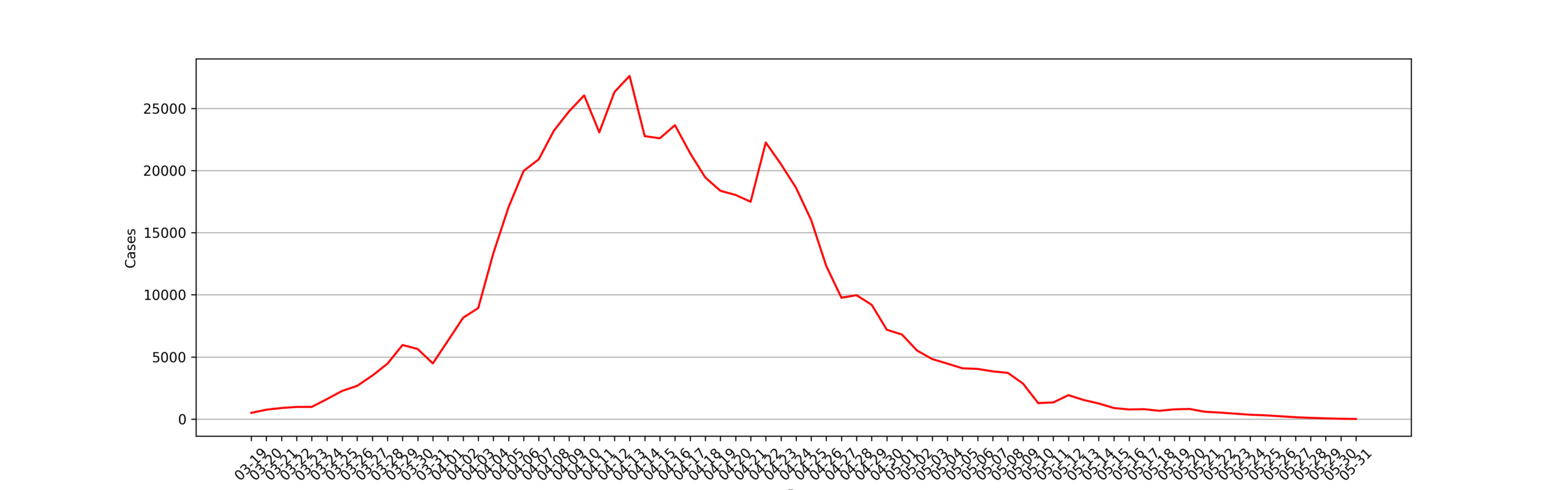
No entire COVID-19 statistics data of the Shanghai lockdown period can be found in the JHU CSSE COVID-19 Data project. Data of project shanghai-lockdown-covid-19 is crawled from Shanghai Government‘s public website, began on 19/03/2022, the date of my place lockdown.
Shanghai is divided by the Huangpu River into two parts, the Pudong area, and the Puxi area. Pudong’s lockdown began on 28/03/2022 firstly, and Puxi started its shutdown on 01/04/2022.
Shanghai Government has announced its city-wide lockdowns will be gradually lifted from 1 June on 16/05/2022, after 15 out of 16 districts achieving “social dynamic Zero-Covid cases”. My place alse reopened on the same day, but with some limits.
Shanghai returned to normal on 1 June, the epidemic wave in the city is under control effectively and this project has stopped updating at 2 June.
Data files can be found in directory data, including:
- JSON
- CSV
- Excel
- Sqlite
Notice: I think db files are too large, and they will make this repo hard to clone. If you want to get the latest db files, uncomment the line in db.py and run the file to generate all db files.
I have disabled the update workflow at 2 June, this project will not be updated anymore.
This project will be updated every 15min between 8am and 10pm GMT+8 by GitHub Actions.
git clone --depeth=1 https://github.com/lewangdev/shanghai-lockdown-covid-19.git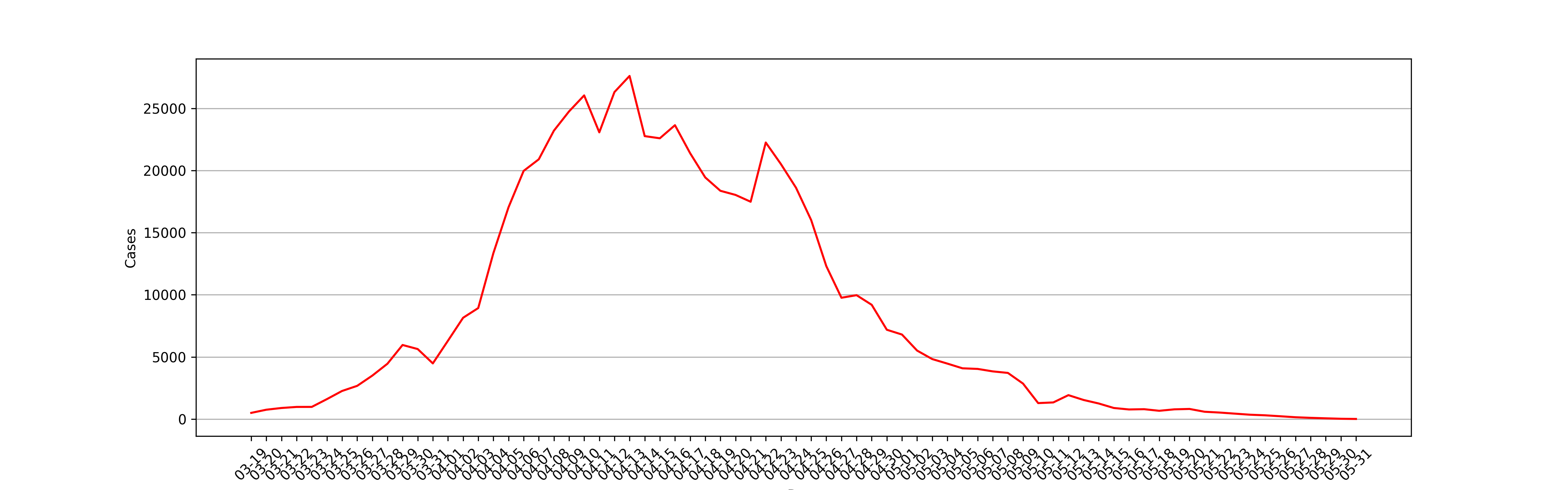
| Date/Details | New Cases(*) | Deaths | Confirmed Cases | Asymptomatic Cases | A2C Cases(*) |
|---|---|---|---|---|---|
| 2022-05-31 | 14 | 0 | 5 | 10 | 1 |
| 2022-05-30 | 29 | 0 | 9 | 22 | 2 |
| 2022-05-29 | 65 | 0 | 6 | 61 | 2 |
| 2022-05-28 | 104 | 0 | 29 | 93 | 18 |
| 2022-05-27 | 152 | 0 | 39 | 131 | 18 |
| 2022-05-26 | 231 | 1 | 45 | 219 | 33 |
| 2022-05-25 | 307 | 1 | 48 | 290 | 31 |
| 2022-05-24 | 355 | 0 | 44 | 343 | 32 |
| 2022-05-23 | 441 | 1 | 58 | 422 | 39 |
| 2022-05-22 | 528 | 1 | 55 | 503 | 30 |
| 2022-05-21 | 593 | 3 | 52 | 570 | 29 |
| 2022-05-20 | 819 | 1 | 84 | 784 | 49 |
| 2022-05-19 | 787 | 0 | 88 | 770 | 71 |
| 2022-05-18 | 671 | 1 | 82 | 637 | 48 |
| 2022-05-17 | 799 | 3 | 96 | 759 | 56 |
| 2022-05-16 | 777 | 1 | 77 | 746 | 46 |
| 2022-05-15 | 896 | 4 | 69 | 869 | 42 |
| 2022-05-14 | 1258 | 3 | 166 | 1203 | 111 |
| 2022-05-13 | 1541 | 1 | 194 | 1487 | 140 |
| 2022-05-12 | 1929 | 2 | 227 | 1869 | 167 |
| 2022-05-11 | 1343 | 5 | 144 | 1305 | 106 |
| 2022-05-10 | 1289 | 7 | 228 | 1259 | 198 |
| 2022-05-09 | 2858 | 6 | 234 | 2780 | 156 |
| 2022-05-08 | 3717 | 11 | 322 | 3625 | 230 |
| 2022-05-07 | 3840 | 8 | 215 | 3760 | 135 |
| 2022-05-06 | 4039 | 13 | 253 | 3961 | 175 |
| 2022-05-05 | 4088 | 12 | 245 | 4024 | 181 |
| 2022-05-04 | 4466 | 13 | 261 | 4390 | 185 |
| 2022-05-03 | 4831 | 16 | 260 | 4722 | 151 |
| 2022-05-02 | 5514 | 20 | 274 | 5395 | 155 |
| 2022-05-01 | 6804 | 32 | 727 | 6606 | 529 |
| 2022-04-30 | 7189 | 38 | 788 | 7084 | 683 |
| 2022-04-29 | 9196 | 47 | 1249 | 8932 | 985 |
| 2022-04-28 | 9970 | 52 | 5487 | 9545 | 5062 |
| 2022-04-27 | 9764 | 47 | 1292 | 9330 | 858 |
| 2022-04-26 | 12309 | 48 | 1606 | 11956 | 1253 |
| 2022-04-25 | 16012 | 52 | 1661 | 15319 | 968 |
| 2022-04-24 | 18609 | 51 | 2472 | 16983 | 846 |
| 2022-04-23 | 20517 | 39 | 1401 | 19657 | 541 |
| 2022-04-22 | 22250 | 12 | 2736 | 20634 | 1120 |
| 2022-04-21 | 17486 | 11 | 1931 | 15698 | 143 |
| 2022-04-20 | 18036 | 8 | 2634 | 15861 | 459 |
| 2022-04-19 | 18368 | 7 | 2494 | 16407 | 533 |
| 2022-04-18 | 19442 | 7 | 3084 | 17332 | 974 |
| 2022-04-17 | 21395 | 3 | 2417 | 19831 | 853 |
| 2022-04-16 | 23643 | 0 | 3238 | 21582 | 1177 |
| 2022-04-15 | 22591 | 0 | 3590 | 19923 | 922 |
| 2022-04-14 | 22765 | 0 | 3200 | 19872 | 307 |
| 2022-04-13 | 27605 | 0 | 2573 | 25146 | 114 |
| 2022-04-12 | 26307 | 0 | 1189 | 25141 | 23 |
| 2022-04-11 | 23069 | 0 | 994 | 22348 | 273 |
| 2022-04-10 | 26040 | 0 | 914 | 25173 | 47 |
| 2022-04-09 | 24752 | 0 | 1006 | 23937 | 191 |
| 2022-04-08 | 23204 | 0 | 1015 | 22609 | 420 |
| 2022-04-07 | 20899 | 0 | 824 | 20398 | 323 |
| 2022-04-06 | 19967 | 0 | 322 | 19660 | 15 |
| 2022-04-05 | 17037 | 0 | 311 | 16766 | 40 |
| 2022-04-04 | 13350 | 0 | 268 | 13086 | 4 |
| 2022-04-03 | 8935 | 0 | 425 | 8581 | 71 |
| 2022-04-02 | 8153 | 0 | 438 | 7788 | 73 |
| 2022-04-01 | 6309 | 0 | 260 | 6051 | 2 |
| 2022-03-31 | 4482 | 0 | 358 | 4144 | 20 |
| 2022-03-30 | 5637 | 0 | 355 | 5298 | 16 |
| 2022-03-29 | 5964 | 0 | 326 | 5656 | 18 |
| 2022-03-28 | 4456 | 0 | 96 | 4381 | 21 |
| 2022-03-27 | 3500 | 0 | 50 | 3450 | 0 |
| 2022-03-26 | 2676 | 0 | 45 | 2631 | 0 |
| 2022-03-25 | 2264 | 0 | 38 | 2231 | 5 |
| 2022-03-24 | 1609 | 0 | 29 | 1580 | 0 |
| 2022-03-23 | 983 | 0 | 4 | 979 | 0 |
| 2022-03-22 | 981 | 0 | 4 | 977 | 0 |
| 2022-03-21 | 896 | 0 | 31 | 865 | 0 |
| 2022-03-20 | 758 | 0 | 24 | 734 | 0 |
| 2022-03-19 | 503 | 0 | 17 | 492 | 6 |
- New Cases = Confirmed Cases + Asymptomatic Cases – A2C Cases
- A2C Cases: Asymptomatic cases that are confirmed
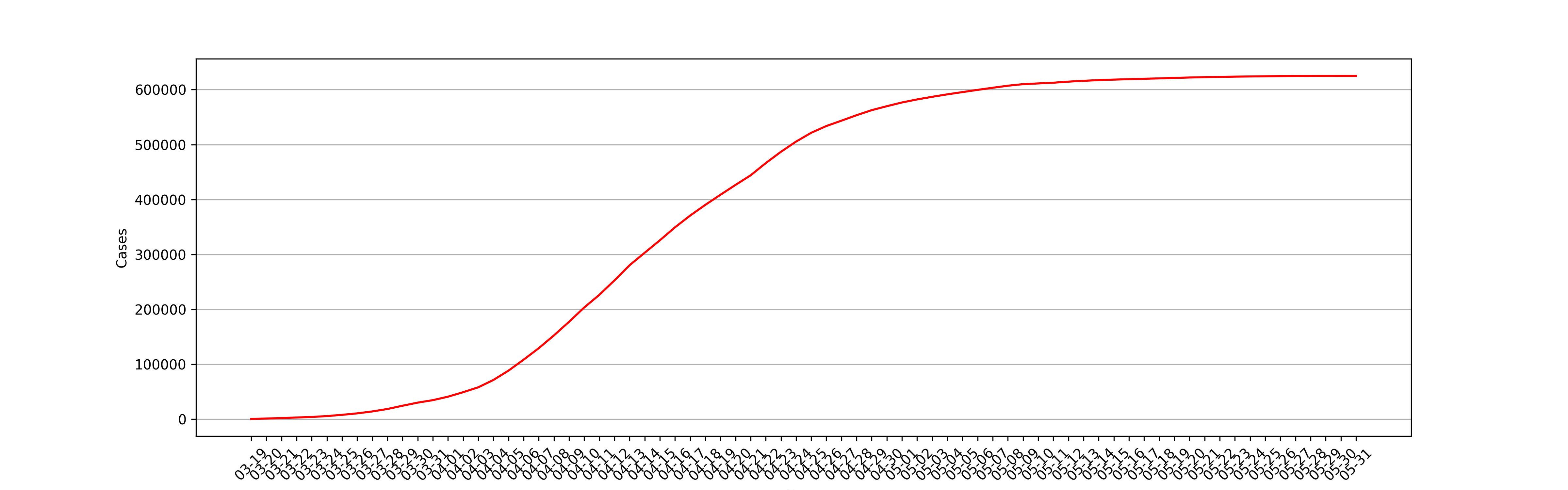
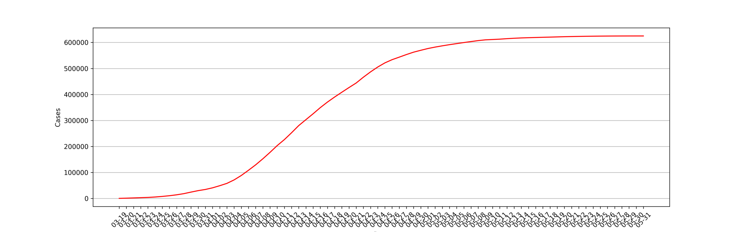
| Date | Total Cases | Total Deaths | Case‑Fatality-Rate |
|---|---|---|---|
| 2022-05-31 | 624963 | 588 | 0.0941% |
| 2022-05-30 | 624949 | 588 | 0.0941% |
| 2022-05-29 | 624920 | 588 | 0.0941% |
| 2022-05-28 | 624855 | 588 | 0.0941% |
| 2022-05-27 | 624751 | 588 | 0.0941% |
| 2022-05-26 | 624599 | 588 | 0.0941% |
| 2022-05-25 | 624368 | 587 | 0.0940% |
| 2022-05-24 | 624061 | 586 | 0.0939% |
| 2022-05-23 | 623706 | 586 | 0.0940% |
| 2022-05-22 | 623265 | 585 | 0.0939% |
| 2022-05-21 | 622737 | 584 | 0.0938% |
| 2022-05-20 | 622144 | 581 | 0.0934% |
| 2022-05-19 | 621325 | 580 | 0.0933% |
| 2022-05-18 | 620538 | 580 | 0.0935% |
| 2022-05-17 | 619867 | 579 | 0.0934% |
| 2022-05-16 | 619068 | 576 | 0.0930% |
| 2022-05-15 | 618291 | 575 | 0.0930% |
| 2022-05-14 | 617395 | 571 | 0.0925% |
| 2022-05-13 | 616137 | 568 | 0.0922% |
| 2022-05-12 | 614596 | 567 | 0.0923% |
| 2022-05-11 | 612667 | 565 | 0.0922% |
| 2022-05-10 | 611324 | 560 | 0.0916% |
| 2022-05-09 | 610035 | 553 | 0.0907% |
| 2022-05-08 | 607177 | 547 | 0.0901% |
| 2022-05-07 | 603460 | 536 | 0.0888% |
| 2022-05-06 | 599620 | 528 | 0.0881% |
| 2022-05-05 | 595581 | 515 | 0.0865% |
| 2022-05-04 | 591493 | 503 | 0.0850% |
| 2022-05-03 | 587027 | 490 | 0.0835% |
| 2022-05-02 | 582196 | 474 | 0.0814% |
| 2022-05-01 | 576682 | 454 | 0.0787% |
| 2022-04-30 | 569878 | 422 | 0.0741% |
| 2022-04-29 | 562689 | 384 | 0.0682% |
| 2022-04-28 | 553493 | 337 | 0.0609% |
| 2022-04-27 | 543523 | 285 | 0.0524% |
| 2022-04-26 | 533759 | 238 | 0.0446% |
| 2022-04-25 | 521450 | 190 | 0.0364% |
| 2022-04-24 | 505438 | 138 | 0.0273% |
| 2022-04-23 | 486829 | 87 | 0.0179% |
| 2022-04-22 | 466312 | 48 | 0.0103% |
| 2022-04-21 | 444062 | 36 | 0.0081% |
| 2022-04-20 | 426576 | 25 | 0.0059% |
| 2022-04-19 | 408540 | 17 | 0.0042% |
| 2022-04-18 | 390172 | 10 | 0.0026% |
| 2022-04-17 | 370730 | 3 | 0.0008% |
| 2022-04-16 | 349335 | 0 | 0.0000% |
| 2022-04-15 | 325692 | 0 | 0.0000% |
| 2022-04-14 | 303101 | 0 | 0.0000% |
| 2022-04-13 | 280336 | 0 | 0.0000% |
| 2022-04-12 | 252731 | 0 | 0.0000% |
| 2022-04-11 | 226424 | 0 | 0.0000% |
| 2022-04-10 | 203355 | 0 | 0.0000% |
| 2022-04-09 | 177315 | 0 | 0.0000% |
| 2022-04-08 | 152563 | 0 | 0.0000% |
| 2022-04-07 | 129359 | 0 | 0.0000% |
| 2022-04-06 | 108460 | 0 | 0.0000% |
| 2022-04-05 | 88493 | 0 | 0.0000% |
| 2022-04-04 | 71456 | 0 | 0.0000% |
| 2022-04-03 | 58106 | 0 | 0.0000% |
| 2022-04-02 | 49171 | 0 | 0.0000% |
| 2022-04-01 | 41018 | 0 | 0.0000% |
| 2022-03-31 | 34709 | 0 | 0.0000% |
| 2022-03-30 | 30227 | 0 | 0.0000% |
| 2022-03-29 | 24590 | 0 | 0.0000% |
| 2022-03-28 | 18626 | 0 | 0.0000% |
| 2022-03-27 | 14170 | 0 | 0.0000% |
| 2022-03-26 | 10670 | 0 | 0.0000% |
| 2022-03-25 | 7994 | 0 | 0.0000% |
| 2022-03-24 | 5730 | 0 | 0.0000% |
| 2022-03-23 | 4121 | 0 | 0.0000% |
| 2022-03-22 | 3138 | 0 | 0.0000% |
| 2022-03-21 | 2157 | 0 | 0.0000% |
| 2022-03-20 | 1261 | 0 | 0.0000% |
| 2022-03-19 | 503 | 0 | 0.0000% |
| Date/District | 浦东新区 | 黄浦区 | 静安区 | 徐汇区 | 长宁区 | 普陀区 | 虹口区 | 杨浦区 | 宝山区 | 闵行区 | 嘉定区 | 金山区 | 松江区 | 青浦区 | 奉贤区 | 崇明区 |
|---|---|---|---|---|---|---|---|---|---|---|---|---|---|---|---|---|
| 2022-05-31 | 4 | 0 | 2 | 0 | 2 | 0 | 3 | 3 | 0 | 0 | 0 | 0 | 0 | 0 | 0 | 0 |
| 2022-05-30 | 6 | 0 | 6 | 0 | 1 | 0 | 6 | 7 | 0 | 4 | 0 | 0 | 1 | 0 | 0 | 0 |
| 2022-05-29 | 12 | 0 | 8 | 5 | 1 | 2 | 8 | 18 | 5 | 4 | 2 | 0 | 0 | 0 | 0 | 0 |
| 2022-05-28 | 18 | 7 | 12 | 10 | 8 | 0 | 14 | 32 | 11 | 8 | 0 | 0 | 0 | 2 | 0 | 0 |
| 2022-05-27 | 28 | 11 | 21 | 12 | 5 | 4 | 20 | 42 | 12 | 6 | 4 | 0 | 0 | 1 | 0 | 0 |
| 2022-05-26 | 35 | 19 | 32 | 18 | 8 | 6 | 30 | 73 | 18 | 15 | 4 | 0 | 2 | 4 | 0 | 0 |
| 2022-05-25 | 44 | 29 | 39 | 21 | 16 | 9 | 41 | 83 | 28 | 21 | 5 | 0 | 0 | 2 | 0 | 0 |
| 2022-05-24 | 47 | 33 | 40 | 22 | 26 | 9 | 54 | 103 | 21 | 24 | 3 | 0 | 1 | 4 | 0 | 0 |
| 2022-05-23 | 60 | 31 | 57 | 27 | 16 | 12 | 88 | 131 | 31 | 14 | 3 | 0 | 7 | 3 | 0 | 0 |
| 2022-05-22 | 59 | 43 | 62 | 42 | 27 | 12 | 116 | 139 | 34 | 15 | 2 | 0 | 5 | 2 | 0 | 0 |
| 2022-05-21 | 75 | 31 | 81 | 42 | 15 | 14 | 129 | 169 | 34 | 12 | 0 | 0 | 13 | 5 | 0 | 0 |
| 2022-05-20 | 78 | 50 | 87 | 41 | 18 | 20 | 142 | 331 | 36 | 36 | 9 | 1 | 6 | 12 | 0 | 0 |
| 2022-05-19 | 82 | 66 | 151 | 37 | 27 | 20 | 121 | 235 | 49 | 33 | 6 | 1 | 10 | 17 | 0 | 0 |
| 2022-05-18 | 75 | 75 | 69 | 44 | 19 | 13 | 74 | 208 | 45 | 52 | 18 | 9 | 15 | 3 | 0 | 0 |
| 2022-05-17 | 83 | 83 | 103 | 51 | 18 | 12 | 59 | 246 | 73 | 59 | 27 | 8 | 19 | 14 | 0 | 0 |
| 2022-05-16 | 89 | 89 | 62 | 52 | 24 | 10 | 49 | 257 | 78 | 48 | 27 | 6 | 11 | 20 | 1 | 0 |
| 2022-05-15 | 98 | 93 | 79 | 63 | 15 | 8 | 69 | 331 | 83 | 35 | 35 | 4 | 14 | 10 | 1 | 0 |
| 2022-05-14 | 150 | 186 | 143 | 89 | 50 | 28 | 67 | 321 | 117 | 81 | 84 | 16 | 6 | 28 | 0 | 1 |
| 2022-05-13 | 187 | 243 | 184 | 105 | 37 | 28 | 91 | 415 | 154 | 129 | 63 | 7 | 11 | 24 | 0 | 3 |
| 2022-05-12 | 280 | 297 | 207 | 93 | 59 | 29 | 103 | 549 | 174 | 143 | 109 | 1 | 22 | 20 | 1 | 9 |
| 2022-05-11 | 250 | 246 | 170 | 74 | 40 | 29 | 102 | 165 | 129 | 91 | 90 | 3 | 14 | 37 | 5 | 4 |
| 2022-05-10 | 263 | 264 | 219 | 83 | 16 | 30 | 136 | 167 | 142 | 79 | 34 | 0 | 19 | 27 | 0 | 8 |
| 2022-05-09 | 588 | 414 | 393 | 128 | 53 | 50 | 269 | 383 | 162 | 328 | 148 | 1 | 26 | 56 | 6 | 9 |
| 2022-05-08 | 692 | 502 | 620 | 306 | 77 | 49 | 317 | 576 | 332 | 225 | 136 | 4 | 40 | 49 | 6 | 16 |
| 2022-05-07 | 675 | 612 | 548 | 299 | 65 | 56 | 272 | 613 | 345 | 227 | 119 | 0 | 48 | 34 | 11 | 51 |
| 2022-05-06 | 584 | 627 | 484 | 330 | 71 | 77 | 279 | 425 | 502 | 309 | 201 | 8 | 27 | 169 | 21 | 100 |
| 2022-05-05 | 677 | 772 | 515 | 323 | 87 | 79 | 267 | 411 | 500 | 235 | 201 | 2 | 83 | 56 | 11 | 50 |
| 2022-05-04 | 889 | 775 | 545 | 330 | 121 | 91 | 326 | 393 | 459 | 285 | 215 | 3 | 92 | 70 | 1 | 56 |
| 2022-05-03 | 883 | 939 | 565 | 363 | 102 | 62 | 358 | 421 | 620 | 252 | 175 | 4 | 90 | 43 | 6 | 99 |
| 2022-05-02 | 1162 | 974 | 616 | 417 | 151 | 79 | 366 | 388 | 636 | 287 | 279 | 7 | 68 | 94 | 10 | 135 |
| 2022-05-01 | 1652 | 1112 | 702 | 442 | 243 | 95 | 669 | 467 | 983 | 386 | 268 | 14 | 96 | 115 | 13 | 76 |
| 2022-04-30 | 1625 | 1156 | 996 | 488 | 181 | 114 | 591 | 342 | 1133 | 431 | 259 | 11 | 105 | 128 | 4 | 308 |
| 2022-04-29 | 2028 | 1399 | 1267 | 602 | 377 | 141 | 1015 | 767 | 1197 | 516 | 268 | 19 | 134 | 156 | 26 | 269 |
| 2022-04-28 | 3472 | 2656 | 1364 | 1580 | 647 | 235 | 1374 | 808 | 1243 | 422 | 488 | 28 | 402 | 269 | 6 | 38 |
| 2022-04-27 | 2993 | 1452 | 1089 | 552 | 208 | 301 | 1091 | 526 | 1115 | 321 | 292 | 41 | 231 | 208 | 3 | 199 |
| 2022-04-26 | 2745 | 1228 | 1394 | 904 | 419 | 365 | 1136 | 1106 | 1976 | 749 | 434 | 28 | 287 | 311 | 13 | 467 |
| 2022-04-25 | 3912 | 2671 | 1016 | 1341 | 534 | 418 | 1270 | 1244 | 1786 | 717 | 543 | 22 | 641 | 379 | 12 | 474 |
| 2022-04-24 | 6181 | 1755 | 1702 | 1396 | 749 | 477 | 655 | 1235 | 2506 | 1229 | 601 | 68 | 548 | 251 | 7 | 95 |
| 2022-04-23 | 7626 | 1959 | 471 | 1722 | 727 | 478 | 819 | 1277 | 2886 | 877 | 751 | 44 | 773 | 424 | 16 | 208 |
| 2022-04-22 | 7961 | 2843 | 786 | 1275 | 713 | 523 | 997 | 1356 | 2033 | 1305 | 500 | 26 | 2568 | 359 | 8 | 117 |
| 2022-04-21 | 4655 | 1752 | 2064 | 1366 | 496 | 489 | 885 | 543 | 978 | 2563 | 776 | 30 | 493 | 385 | 34 | 120 |
| 2022-04-20 | 4465 | 3097 | 1130 | 1447 | 726 | 555 | 832 | 2005 | 833 | 1686 | 649 | 17 | 676 | 280 | 32 | 65 |
| 2022-04-19 | 5646 | 3084 | 1733 | 1608 | 618 | 528 | 753 | 766 | 957 | 1602 | 743 | 9 | 325 | 389 | 60 | 80 |
| 2022-04-18 | 8831 | 3323 | 1010 | 572 | 680 | 371 | 1092 | 481 | 1030 | 1372 | 588 | 7 | 762 | 257 | 14 | 26 |
| 2022-04-17 | 7740 | 1896 | 842 | 1553 | 739 | 1225 | 1166 | 887 | 1450 | 2402 | 978 | 24 | 905 | 369 | 20 | 52 |
| 2022-04-16 | 10791 | 1565 | 1134 | 1532 | 706 | 1331 | 1027 | 860 | 1293 | 3060 | 685 | 21 | 410 | 305 | 51 | 49 |
| 2022-04-15 | 10282 | 1384 | 433 | 1689 | 752 | 426 | 1497 | 1411 | 1323 | 2037 | 741 | 31 | 773 | 536 | 106 | 92 |
| 2022-04-14 | 11656 | 2013 | 266 | 1342 | 998 | 264 | 930 | 817 | 417 | 2378 | 803 | 28 | 761 | 304 | 35 | 60 |
| 2022-04-13 | 15027 | 1408 | 220 | 1492 | 957 | 475 | 1488 | 1185 | 651 | 2939 | 721 | 34 | 657 | 319 | 83 | 63 |
| 2022-04-12 | 11049 | 1804 | 1056 | 1108 | 1133 | 1170 | 931 | 1159 | 295 | 4245 | 986 | 39 | 712 | 524 | 33 | 86 |
| 2022-04-11 | 8306 | 2223 | 552 | 1771 | 393 | 1878 | 1375 | 1420 | 1024 | 3007 | 208 | 38 | 691 | 331 | 68 | 57 |
| 2022-04-10 | 6732 | 1761 | 603 | 3203 | 387 | 1001 | 1238 | 1877 | 1839 | 3189 | 1405 | 57 | 1825 | 877 | 38 | 55 |
| 2022-04-09 | 11130 | 548 | 602 | 1150 | 757 | 653 | 349 | 1080 | 2261 | 4624 | 369 | 68 | 500 | 557 | 124 | 171 |
| 2022-04-08 | 7286 | 2607 | 665 | 1629 | 614 | 1094 | 378 | 701 | 2821 | 2854 | 1505 | 90 | 771 | 342 | 97 | 170 |
| 2022-04-07 | 9050 | 1380 | 381 | 2076 | 852 | 957 | 594 | 601 | 414 | 2257 | 933 | 129 | 751 | 493 | 92 | 262 |
| 2022-04-06 | 8457 | 1044 | 545 | 1107 | 350 | 1033 | 668 | 630 | 660 | 2409 | 1408 | 79 | 781 | 470 | 278 | 63 |
| 2022-04-05 | 8145 | 658 | 302 | 920 | 84 | 483 | 410 | 623 | 554 | 2937 | 481 | 77 | 796 | 384 | 144 | 79 |
| 2022-04-04 | 7071 | 970 | 50 | 1229 | 33 | 254 | 608 | 220 | 265 | 1381 | 237 | 52 | 559 | 314 | 64 | 47 |
| 2022-04-03 | 3654 | 824 | 338 | 499 | 104 | 321 | 188 | 374 | 467 | 940 | 415 | 103 | 263 | 232 | 119 | 165 |
| 2022-04-02 | 2038 | 659 | 324 | 1042 | 100 | 388 | 342 | 274 | 485 | 829 | 617 | 60 | 567 | 231 | 157 | 113 |
| 2022-04-01 | 2584 | 2584 | 260 | 260 | 189 | 189 | 639 | 639 | 37 | 37 | 245 | 245 | 61 | 61 | 134 | 134 |
| 2022-03-31 | 2407 | 121 | 164 | 226 | 256 | 15 | 128 | 174 | 17 | 392 | 54 | 42 | 184 | 95 | 183 | 44 |
| 2022-03-30 | 2207 | 361 | 102 | 404 | 128 | 146 | 84 | 100 | 504 | 780 | 158 | 33 | 246 | 77 | 130 | 193 |
| 2022-03-29 | 2183 | 110 | 175 | 1100 | 30 | 113 | 73 | 99 | 363 | 988 | 255 | 26 | 229 | 87 | 96 | 55 |
| 2022-03-28 | 2506 | 283 | 104 | 91 | 115 | 81 | 8 | 47 | 311 | 370 | 209 | 19 | 94 | 57 | 115 | 67 |
| 2022-03-27 | 1429 | 56 | 70 | 277 | 45 | 70 | 27 | 35 | 94 | 619 | 251 | 13 | 190 | 43 | 45 | 236 |
| 2022-03-26 | 323 | 160 | 108 | 331 | 29 | 69 | 50 | 23 | 153 | 972 | 242 | 4 | 79 | 22 | 84 | 27 |
| 2022-03-25 | 1914 | 23 | 2 | 3 | 4 | 9 | 4 | 11 | 4 | 206 | 19 | 1 | 15 | 13 | 0 | 41 |
| 2022-03-24 | 193 | 102 | 70 | 167 | 59 | 38 | 29 | 21 | 87 | 490 | 130 | 12 | 92 | 13 | 24 | 82 |
| 2022-03-23 | 218 | 20 | 48 | 106 | 11 | 34 | 26 | 11 | 69 | 256 | 69 | 5 | 34 | 10 | 12 | 54 |
| 2022-03-22 | 237 | 59 | 28 | 87 | 19 | 21 | 13 | 3 | 16 | 305 | 111 | 4 | 31 | 20 | 8 | 19 |
| 2022-03-21 | 169 | 49 | 44 | 130 | 26 | 31 | 23 | 10 | 67 | 122 | 103 | 16 | 39 | 5 | 22 | 40 |
| 2022-03-20 | 220 | 42 | 32 | 46 | 13 | 18 | 12 | 8 | 13 | 265 | 40 | 11 | 9 | 4 | 13 | 0 |
| 2022-03-19 | 135 | 36 | 15 | 61 | 12 | 25 | 0 | 14 | 17 | 53 | 81 | 3 | 16 | 5 | 6 | 23 |
| Date/District | 浦东新区 | 黄浦区 | 静安区 | 徐汇区 | 长宁区 | 普陀区 | 虹口区 | 杨浦区 | 宝山区 | 闵行区 | 嘉定区 | 金山区 | 松江区 | 青浦区 | 奉贤区 | 崇明区 |
|---|---|---|---|---|---|---|---|---|---|---|---|---|---|---|---|---|
| 2022-05-31 | 229688 | 61684 | 32497 | 46371 | 18273 | 20041 | 30943 | 35501 | 43510 | 66625 | 23773 | 1666 | 22657 | 11930 | 2897 | 5716 |
| 2022-05-30 | 229684 | 61684 | 32495 | 46371 | 18271 | 20041 | 30940 | 35498 | 43510 | 66625 | 23773 | 1666 | 22657 | 11930 | 2897 | 5716 |
| 2022-05-29 | 229678 | 61684 | 32489 | 46371 | 18270 | 20041 | 30934 | 35491 | 43510 | 66621 | 23773 | 1666 | 22656 | 11930 | 2897 | 5716 |
| 2022-05-28 | 229666 | 61684 | 32481 | 46366 | 18269 | 20039 | 30926 | 35473 | 43505 | 66617 | 23771 | 1666 | 22656 | 11930 | 2897 | 5716 |
| 2022-05-27 | 229648 | 61677 | 32469 | 46356 | 18261 | 20039 | 30912 | 35441 | 43494 | 66609 | 23771 | 1666 | 22656 | 11928 | 2897 | 5716 |
| 2022-05-26 | 229620 | 61666 | 32448 | 46344 | 18256 | 20035 | 30892 | 35399 | 43482 | 66603 | 23767 | 1666 | 22656 | 11927 | 2897 | 5716 |
| 2022-05-25 | 229585 | 61647 | 32416 | 46326 | 18248 | 20029 | 30862 | 35326 | 43464 | 66588 | 23763 | 1666 | 22654 | 11923 | 2897 | 5716 |
| 2022-05-24 | 229541 | 61618 | 32377 | 46305 | 18232 | 20020 | 30821 | 35243 | 43436 | 66567 | 23758 | 1666 | 22654 | 11921 | 2897 | 5716 |
| 2022-05-23 | 229494 | 61585 | 32337 | 46283 | 18206 | 20011 | 30767 | 35140 | 43415 | 66543 | 23755 | 1666 | 22653 | 11917 | 2897 | 5716 |
| 2022-05-22 | 229434 | 61554 | 32280 | 46256 | 18190 | 19999 | 30679 | 35009 | 43384 | 66529 | 23752 | 1666 | 22646 | 11914 | 2897 | 5716 |
| 2022-05-21 | 229375 | 61511 | 32218 | 46214 | 18163 | 19987 | 30563 | 34870 | 43350 | 66514 | 23750 | 1666 | 22641 | 11912 | 2897 | 5716 |
| 2022-05-20 | 229300 | 61480 | 32137 | 46172 | 18148 | 19973 | 30434 | 34701 | 43316 | 66502 | 23750 | 1666 | 22628 | 11907 | 2897 | 5716 |
| 2022-05-19 | 229222 | 61430 | 32050 | 46131 | 18130 | 19953 | 30292 | 34370 | 43280 | 66466 | 23741 | 1665 | 22622 | 11895 | 2897 | 5716 |
| 2022-05-18 | 229140 | 61364 | 31899 | 46094 | 18103 | 19933 | 30171 | 34135 | 43231 | 66433 | 23735 | 1664 | 22612 | 11878 | 2897 | 5716 |
| 2022-05-17 | 229065 | 61289 | 31830 | 46050 | 18084 | 19920 | 30097 | 33927 | 43186 | 66381 | 23717 | 1655 | 22597 | 11875 | 2897 | 5716 |
| 2022-05-16 | 228982 | 61206 | 31727 | 45999 | 18066 | 19908 | 30038 | 33681 | 43113 | 66322 | 23690 | 1647 | 22578 | 11861 | 2897 | 5716 |
| 2022-05-15 | 228893 | 61117 | 31665 | 45947 | 18042 | 19898 | 29989 | 33424 | 43035 | 66274 | 23663 | 1641 | 22567 | 11841 | 2896 | 5716 |
| 2022-05-14 | 228795 | 61024 | 31586 | 45884 | 18027 | 19890 | 29920 | 33093 | 42952 | 66239 | 23628 | 1637 | 22553 | 11831 | 2895 | 5716 |
| 2022-05-13 | 228645 | 60838 | 31443 | 45795 | 17977 | 19862 | 29853 | 32772 | 42835 | 66158 | 23544 | 1621 | 22547 | 11803 | 2895 | 5715 |
| 2022-05-12 | 228458 | 60595 | 31259 | 45690 | 17940 | 19834 | 29762 | 32357 | 42681 | 66029 | 23481 | 1614 | 22536 | 11779 | 2895 | 5712 |
| 2022-05-11 | 228178 | 60298 | 31052 | 45597 | 17881 | 19805 | 29659 | 31808 | 42507 | 65886 | 23372 | 1613 | 22514 | 11759 | 2894 | 5703 |
| 2022-05-10 | 227928 | 60052 | 30882 | 45523 | 17841 | 19776 | 29557 | 31643 | 42378 | 65795 | 23282 | 1610 | 22500 | 11722 | 2889 | 5699 |
| 2022-05-09 | 227665 | 59788 | 30663 | 45440 | 17825 | 19746 | 29421 | 31476 | 42236 | 65716 | 23248 | 1610 | 22481 | 11695 | 2889 | 5691 |
| 2022-05-08 | 227077 | 59374 | 30270 | 45312 | 17772 | 19696 | 29152 | 31093 | 42074 | 65388 | 23100 | 1609 | 22455 | 11639 | 2883 | 5682 |
| 2022-05-07 | 226385 | 58872 | 29650 | 45006 | 17695 | 19647 | 28835 | 30517 | 41742 | 65163 | 22964 | 1605 | 22415 | 11590 | 2877 | 5666 |
| 2022-05-06 | 225710 | 58260 | 29102 | 44707 | 17630 | 19591 | 28563 | 29904 | 41397 | 64936 | 22845 | 1605 | 22367 | 11556 | 2866 | 5615 |
| 2022-05-05 | 225126 | 57633 | 28618 | 44377 | 17559 | 19514 | 28284 | 29479 | 40895 | 64627 | 22644 | 1597 | 22340 | 11387 | 2845 | 5515 |
| 2022-05-04 | 224449 | 56861 | 28103 | 44054 | 17472 | 19435 | 28017 | 29068 | 40395 | 64392 | 22443 | 1595 | 22257 | 11331 | 2834 | 5465 |
| 2022-05-03 | 223560 | 56086 | 27558 | 43724 | 17351 | 19344 | 27691 | 28675 | 39936 | 64107 | 22228 | 1592 | 22165 | 11261 | 2833 | 5409 |
| 2022-05-02 | 222677 | 55147 | 26993 | 43361 | 17249 | 19282 | 27333 | 28254 | 39316 | 63855 | 22053 | 1588 | 22075 | 11218 | 2827 | 5310 |
| 2022-05-01 | 221515 | 54173 | 26377 | 42944 | 17098 | 19203 | 26967 | 27866 | 38680 | 63568 | 21774 | 1581 | 22007 | 11124 | 2817 | 5175 |
| 2022-04-30 | 219863 | 53061 | 25675 | 42502 | 16855 | 19108 | 26298 | 27399 | 37697 | 63182 | 21506 | 1567 | 21911 | 11009 | 2804 | 5099 |
| 2022-04-29 | 218238 | 51905 | 24679 | 42014 | 16674 | 18994 | 25707 | 27057 | 36564 | 62751 | 21247 | 1556 | 21806 | 10881 | 2800 | 4791 |
| 2022-04-28 | 216210 | 50506 | 23412 | 41412 | 16297 | 18853 | 24692 | 26290 | 35367 | 62235 | 20979 | 1537 | 21672 | 10725 | 2774 | 4522 |
| 2022-04-27 | 212738 | 47850 | 22048 | 39832 | 15650 | 18618 | 23318 | 25482 | 34124 | 61813 | 20491 | 1509 | 21270 | 10456 | 2768 | 4484 |
| 2022-04-26 | 209745 | 46398 | 20959 | 39280 | 15442 | 18317 | 22227 | 24956 | 33009 | 61492 | 20199 | 1468 | 21039 | 10248 | 2765 | 4285 |
| 2022-04-25 | 207000 | 45170 | 19565 | 38376 | 15023 | 17952 | 21091 | 23850 | 31033 | 60743 | 19765 | 1440 | 20752 | 9937 | 2752 | 3818 |
| 2022-04-24 | 203088 | 42499 | 18549 | 37035 | 14489 | 17534 | 19821 | 22606 | 29247 | 60026 | 19222 | 1418 | 20111 | 9558 | 2740 | 3344 |
| 2022-04-23 | 196907 | 40744 | 16847 | 35639 | 13740 | 17057 | 19166 | 21371 | 26741 | 58797 | 18621 | 1350 | 19563 | 9307 | 2733 | 3249 |
| 2022-04-22 | 189281 | 38785 | 16376 | 33917 | 13013 | 16579 | 18347 | 20094 | 23855 | 57920 | 17870 | 1306 | 18790 | 8883 | 2717 | 3041 |
| 2022-04-21 | 181320 | 35942 | 15590 | 32642 | 12300 | 16056 | 17350 | 18738 | 21822 | 56615 | 17370 | 1280 | 16222 | 8524 | 2709 | 2924 |
| 2022-04-20 | 176665 | 34190 | 13526 | 31276 | 11804 | 15567 | 16465 | 18195 | 20844 | 54052 | 16594 | 1250 | 15729 | 8139 | 2675 | 2804 |
| 2022-04-19 | 172200 | 31093 | 12396 | 29829 | 11078 | 15012 | 15633 | 16190 | 20011 | 52366 | 15945 | 1233 | 15053 | 7859 | 2643 | 2739 |
| 2022-04-18 | 166554 | 28009 | 10663 | 28221 | 10460 | 14484 | 14880 | 15424 | 19054 | 50764 | 15202 | 1224 | 14728 | 7470 | 2583 | 2659 |
| 2022-04-17 | 157723 | 24686 | 9653 | 27649 | 9780 | 14113 | 13788 | 14943 | 18024 | 49392 | 14614 | 1217 | 13966 | 7213 | 2569 | 2633 |
| 2022-04-16 | 149983 | 22790 | 8811 | 26096 | 9041 | 12888 | 12622 | 14056 | 16574 | 46990 | 13636 | 1193 | 13061 | 6844 | 2549 | 2581 |
| 2022-04-15 | 139192 | 21225 | 7677 | 24564 | 8335 | 11557 | 11595 | 13196 | 15281 | 43930 | 12951 | 1172 | 12651 | 6539 | 2498 | 2532 |
| 2022-04-14 | 128910 | 19841 | 7244 | 22875 | 7583 | 11131 | 10098 | 11785 | 13958 | 41893 | 12210 | 1141 | 11878 | 6003 | 2392 | 2440 |
| 2022-04-13 | 117254 | 17828 | 6978 | 21533 | 6585 | 10867 | 9168 | 10968 | 13541 | 39515 | 11407 | 1113 | 11117 | 5699 | 2357 | 2380 |
| 2022-04-12 | 102227 | 16420 | 6758 | 20041 | 5628 | 10392 | 7680 | 9783 | 12890 | 36576 | 10686 | 1079 | 10460 | 5380 | 2274 | 2317 |
| 2022-04-11 | 91178 | 14616 | 5702 | 18933 | 4495 | 9222 | 6749 | 8624 | 12595 | 32331 | 9700 | 1040 | 9748 | 4856 | 2241 | 2231 |
| 2022-04-10 | 82872 | 12393 | 5150 | 17162 | 4102 | 7344 | 5374 | 7204 | 11571 | 29324 | 9492 | 1002 | 9057 | 4525 | 2173 | 2174 |
| 2022-04-09 | 76140 | 10632 | 4547 | 13959 | 3715 | 6343 | 4136 | 5327 | 9732 | 26135 | 8087 | 945 | 7232 | 3648 | 2135 | 2119 |
| 2022-04-08 | 65010 | 10084 | 3945 | 12809 | 2958 | 5690 | 3787 | 4247 | 7471 | 21511 | 7718 | 877 | 6732 | 3091 | 2011 | 1948 |
| 2022-04-07 | 57724 | 7477 | 3280 | 11180 | 2344 | 4596 | 3409 | 3546 | 4650 | 18657 | 6213 | 787 | 5961 | 2749 | 1914 | 1778 |
| 2022-04-06 | 48674 | 6097 | 2899 | 9104 | 1492 | 3639 | 2815 | 2945 | 4236 | 16400 | 5280 | 658 | 5210 | 2256 | 1822 | 1516 |
| 2022-04-05 | 40217 | 5053 | 2354 | 7997 | 1142 | 2606 | 2147 | 2315 | 3576 | 13991 | 3872 | 579 | 4429 | 1786 | 1544 | 1453 |
| 2022-04-04 | 32072 | 4395 | 2052 | 7077 | 1058 | 2123 | 1737 | 1692 | 3022 | 11054 | 3391 | 502 | 3633 | 1402 | 1400 | 1374 |
| 2022-04-03 | 25001 | 3425 | 2002 | 5848 | 1025 | 1869 | 1129 | 1472 | 2757 | 9673 | 3154 | 450 | 3074 | 1088 | 1336 | 1327 |
| 2022-04-02 | 21347 | 2601 | 1664 | 5349 | 921 | 1548 | 941 | 1098 | 2290 | 8733 | 2739 | 347 | 2811 | 856 | 1217 | 1162 |
| 2022-04-01 | 16725 | 19309 | 1682 | 1942 | 1151 | 1340 | 3668 | 4307 | 784 | 821 | 915 | 1160 | 538 | 599 | 690 | 824 |
| 2022-03-31 | 14141 | 1422 | 962 | 3029 | 747 | 670 | 477 | 556 | 1715 | 5818 | 1722 | 189 | 1258 | 451 | 738 | 881 |
| 2022-03-30 | 11734 | 1301 | 798 | 2803 | 491 | 655 | 349 | 382 | 1698 | 5426 | 1668 | 147 | 1074 | 356 | 555 | 837 |
| 2022-03-29 | 9527 | 940 | 696 | 2399 | 363 | 509 | 265 | 282 | 1194 | 4646 | 1510 | 114 | 828 | 279 | 425 | 644 |
| 2022-03-28 | 7344 | 830 | 521 | 1299 | 333 | 396 | 192 | 183 | 831 | 3658 | 1255 | 88 | 599 | 192 | 329 | 589 |
| 2022-03-27 | 4838 | 547 | 417 | 1208 | 218 | 315 | 184 | 136 | 520 | 3288 | 1046 | 69 | 505 | 135 | 214 | 522 |
| 2022-03-26 | 3409 | 491 | 347 | 931 | 173 | 245 | 157 | 101 | 426 | 2669 | 795 | 56 | 315 | 92 | 169 | 286 |
| 2022-03-25 | 3086 | 331 | 239 | 600 | 144 | 176 | 107 | 78 | 273 | 1697 | 553 | 52 | 236 | 70 | 85 | 259 |
| 2022-03-24 | 1172 | 308 | 237 | 597 | 140 | 167 | 103 | 67 | 269 | 1491 | 534 | 51 | 221 | 57 | 85 | 218 |
| 2022-03-23 | 979 | 206 | 167 | 430 | 81 | 129 | 74 | 46 | 182 | 1001 | 404 | 39 | 129 | 44 | 61 | 136 |
| 2022-03-22 | 761 | 186 | 119 | 324 | 70 | 95 | 48 | 35 | 113 | 745 | 335 | 34 | 95 | 34 | 49 | 82 |
| 2022-03-21 | 524 | 127 | 91 | 237 | 51 | 74 | 35 | 32 | 97 | 440 | 224 | 30 | 64 | 14 | 41 | 63 |
| 2022-03-20 | 355 | 78 | 47 | 107 | 25 | 43 | 12 | 22 | 30 | 318 | 121 | 14 | 25 | 9 | 19 | 23 |
| 2022-03-19 | 135 | 36 | 15 | 61 | 12 | 25 | 0 | 14 | 17 | 53 | 81 | 3 | 16 | 5 | 6 | 23 |
| Date/District | 浦东新区 | 黄浦区 | 静安区 | 徐汇区 | 长宁区 | 普陀区 | 虹口区 | 杨浦区 | 宝山区 | 闵行区 | 嘉定区 | 金山区 | 松江区 | 青浦区 | 奉贤区 | 崇明区 |
|---|---|---|---|---|---|---|---|---|---|---|---|---|---|---|---|---|
| 2022-05-31 | 4 | 1 | 1 | 0 | 2 | 0 | 2 | 0 | 0 | 0 | 0 | 0 | 0 | 0 | 0 | 1 |
| 2022-05-30 | 6 | 0 | 5 | 0 | 1 | 0 | 3 | 2 | 0 | 2 | 0 | 0 | 1 | 0 | 0 | 1 |
| 2022-05-29 | 7 | 0 | 4 | 2 | 1 | 1 | 7 | 3 | 4 | 1 | 1 | 0 | 2 | 0 | 0 | 0 |
| 2022-05-28 | 9 | 4 | 9 | 7 | 1 | 0 | 10 | 6 | 7 | 1 | 0 | 0 | 0 | 2 | 0 | 0 |
| 2022-05-27 | 20 | 6 | 14 | 4 | 4 | 2 | 15 | 5 | 9 | 0 | 2 | 0 | 1 | 1 | 0 | 0 |
| 2022-05-26 | 17 | 17 | 13 | 8 | 6 | 3 | 21 | 11 | 11 | 3 | 1 | 0 | 1 | 4 | 0 | 0 |
| 2022-05-25 | 21 | 15 | 22 | 7 | 4 | 7 | 31 | 11 | 17 | 2 | 3 | 0 | 0 | 2 | 0 | 0 |
| 2022-05-24 | 23 | 18 | 23 | 8 | 8 | 4 | 31 | 17 | 15 | 3 | 2 | 0 | 1 | 1 | 0 | 0 |
| 2022-05-23 | 22 | 21 | 19 | 9 | 4 | 6 | 50 | 20 | 20 | 2 | 1 | 0 | 4 | 3 | 0 | 0 |
| 2022-05-22 | 32 | 29 | 28 | 11 | 10 | 6 | 66 | 14 | 21 | 3 | 0 | 0 | 3 | 2 | 0 | 0 |
| 2022-05-21 | 31 | 23 | 33 | 9 | 3 | 9 | 76 | 28 | 23 | 6 | 0 | 0 | 5 | 4 | 0 | 0 |
| 2022-05-20 | 39 | 32 | 47 | 17 | 6 | 12 | 80 | 26 | 21 | 5 | 1 | 1 | 3 | 7 | 0 | 0 |
| 2022-05-19 | 44 | 43 | 68 | 7 | 8 | 14 | 66 | 35 | 34 | 6 | 0 | 0 | 7 | 7 | 0 | 0 |
| 2022-05-18 | 33 | 40 | 26 | 16 | 11 | 8 | 43 | 45 | 33 | 16 | 2 | 0 | 6 | 2 | 0 | 0 |
| 2022-05-17 | 36 | 56 | 29 | 7 | 7 | 9 | 36 | 43 | 42 | 16 | 2 | 0 | 7 | 9 | 0 | 0 |
| 2022-05-16 | 31 | 58 | 29 | 11 | 8 | 7 | 33 | 82 | 43 | 4 | 1 | 2 | 6 | 8 | 0 | 0 |
| 2022-05-15 | 47 | 57 | 13 | 23 | 5 | 5 | 41 | 104 | 51 | 4 | 1 | 2 | 7 | 8 | 1 | 0 |
| 2022-05-14 | 66 | 109 | 67 | 28 | 22 | 21 | 52 | 100 | 59 | 19 | 5 | 2 | 3 | 8 | 0 | 1 |
| 2022-05-13 | 83 | 141 | 76 | 32 | 13 | 17 | 59 | 102 | 76 | 25 | 6 | 0 | 5 | 10 | 0 | 3 |
| 2022-05-12 | 116 | 158 | 80 | 25 | 31 | 15 | 56 | 117 | 93 | 26 | 10 | 0 | 11 | 9 | 0 | 3 |
| 2022-05-11 | 98 | 134 | 87 | 23 | 10 | 16 | 52 | 66 | 72 | 5 | 10 | 0 | 5 | 13 | 1 | 3 |
| 2022-05-10 | 92 | 141 | 108 | 24 | 7 | 19 | 63 | 28 | 88 | 6 | 5 | 0 | 13 | 10 | 0 | 3 |
| 2022-05-09 | 236 | 208 | 161 | 26 | 31 | 31 | 126 | 92 | 65 | 43 | 27 | 0 | 20 | 23 | 3 | 4 |
| 2022-05-08 | 263 | 254 | 231 | 71 | 30 | 27 | 148 | 135 | 169 | 38 | 17 | 0 | 22 | 25 | 0 | 7 |
| 2022-05-07 | 208 | 323 | 226 | 63 | 30 | 28 | 146 | 156 | 169 | 33 | 18 | 0 | 31 | 13 | 2 | 5 |
| 2022-05-06 | 269 | 294 | 231 | 74 | 32 | 34 | 120 | 115 | 234 | 45 | 32 | 1 | 16 | 24 | 1 | 7 |
| 2022-05-05 | 266 | 377 | 206 | 78 | 40 | 47 | 132 | 123 | 224 | 50 | 40 | 0 | 43 | 20 | 2 | 8 |
| 2022-05-04 | 337 | 364 | 225 | 90 | 48 | 36 | 113 | 127 | 209 | 56 | 53 | 0 | 54 | 19 | 0 | 8 |
| 2022-05-03 | 337 | 411 | 247 | 77 | 49 | 23 | 182 | 158 | 232 | 67 | 20 | 0 | 39 | 19 | 3 | 11 |
| 2022-05-02 | 409 | 427 | 236 | 89 | 67 | 38 | 173 | 127 | 262 | 69 | 48 | 0 | 28 | 22 | 3 | 8 |
| 2022-05-01 | 513 | 485 | 234 | 113 | 60 | 39 | 250 | 192 | 326 | 88 | 44 | 0 | 42 | 37 | 0 | 9 |
| 2022-04-30 | 440 | 489 | 313 | 116 | 68 | 46 | 209 | 141 | 388 | 88 | 50 | 0 | 49 | 35 | 0 | 4 |
| 2022-04-29 | 658 | 508 | 407 | 180 | 95 | 41 | 285 | 247 | 386 | 125 | 68 | 2 | 58 | 29 | 2 | 7 |
| 2022-04-28 | 689 | 575 | 361 | 298 | 130 | 79 | 341 | 213 | 277 | 100 | 107 | 1 | 68 | 50 | 0 | 6 |
| 2022-04-27 | 741 | 609 | 403 | 133 | 76 | 99 | 361 | 220 | 312 | 98 | 73 | 0 | 93 | 50 | 2 | 4 |
| 2022-04-26 | 740 | 522 | 376 | 269 | 137 | 106 | 355 | 339 | 515 | 197 | 113 | 1 | 91 | 63 | 5 | 2 |
| 2022-04-25 | 926 | 895 | 305 | 310 | 135 | 119 | 428 | 342 | 388 | 199 | 162 | 0 | 144 | 99 | 3 | 0 |
| 2022-04-24 | 1320 | 718 | 542 | 375 | 179 | 138 | 240 | 378 | 586 | 327 | 184 | 4 | 88 | 58 | 4 | 0 |
| 2022-04-23 | 1472 | 748 | 127 | 308 | 206 | 119 | 297 | 391 | 743 | 225 | 169 | 3 | 168 | 90 | 5 | 0 |
| 2022-04-22 | 1522 | 930 | 238 | 321 | 185 | 112 | 390 | 362 | 556 | 328 | 156 | 1 | 119 | 85 | 0 | 0 |
| 2022-04-21 | 1050 | 658 | 516 | 359 | 157 | 131 | 343 | 200 | 308 | 511 | 174 | 1 | 149 | 94 | 0 | 0 |
| 2022-04-20 | 982 | 948 | 368 | 380 | 206 | 128 | 347 | 482 | 325 | 411 | 179 | 1 | 196 | 60 | 0 | 0 |
| 2022-04-19 | 1144 | 953 | 509 | 360 | 196 | 152 | 284 | 275 | 295 | 391 | 169 | 2 | 92 | 93 | 0 | 0 |
| 2022-04-18 | 1397 | 915 | 290 | 171 | 192 | 130 | 433 | 179 | 346 | 328 | 185 | 0 | 201 | 52 | 1 | 0 |
| 2022-04-17 | 1550 | 681 | 292 | 349 | 174 | 206 | 398 | 300 | 413 | 506 | 204 | 0 | 162 | 85 | 5 | 0 |
| 2022-04-16 | 1778 | 570 | 320 | 374 | 178 | 280 | 365 | 307 | 333 | 562 | 177 | 1 | 52 | 62 | 4 | 4 |
| 2022-04-15 | 1746 | 601 | 106 | 357 | 283 | 64 | 377 | 402 | 234 | 433 | 211 | 2 | 207 | 112 | 11 | 7 |
| 2022-04-14 | 1704 | 700 | 96 | 360 | 298 | 79 | 330 | 302 | 195 | 530 | 219 | 3 | 189 | 58 | 5 | 5 |
| 2022-04-13 | 1863 | 516 | 87 | 365 | 315 | 127 | 522 | 381 | 231 | 623 | 192 | 4 | 221 | 77 | 10 | 6 |
| 2022-04-12 | 1580 | 637 | 395 | 320 | 315 | 271 | 335 | 376 | 141 | 740 | 253 | 7 | 243 | 152 | 12 | 6 |
| 2022-04-11 | 1588 | 668 | 210 | 353 | 159 | 343 | 454 | 453 | 359 | 618 | 65 | 8 | 214 | 91 | 29 | 11 |
| 2022-04-10 | 1421 | 647 | 214 | 585 | 164 | 247 | 380 | 573 | 580 | 505 | 332 | 20 | 381 | 224 | 21 | 6 |
| 2022-04-09 | 1969 | 289 | 232 | 323 | 277 | 220 | 171 | 403 | 786 | 366 | 115 | 12 | 181 | 191 | 28 | 2 |
| 2022-04-08 | 1227 | 825 | 249 | 393 | 235 | 277 | 188 | 281 | 849 | 320 | 381 | 12 | 270 | 112 | 32 | 9 |
| 2022-04-07 | 1706 | 568 | 166 | 325 | 325 | 269 | 132 | 235 | 224 | 287 | 309 | 25 | 284 | 165 | 42 | 10 |
| 2022-04-06 | 1509 | 481 | 227 | 339 | 197 | 289 | 271 | 302 | 323 | 321 | 465 | 33 | 236 | 191 | 75 | 16 |
| 2022-04-05 | 1274 | 339 | 155 | 300 | 55 | 179 | 163 | 276 | 252 | 324 | 135 | 32 | 278 | 179 | 64 | 13 |
| 2022-04-04 | 1443 | 467 | 18 | 403 | 30 | 104 | 261 | 134 | 148 | 162 | 98 | 28 | 209 | 138 | 39 | 9 |
| 2022-04-03 | 1010 | 369 | 168 | 174 | 51 | 135 | 123 | 216 | 207 | 196 | 148 | 53 | 119 | 114 | 72 | 19 |
| 2022-04-02 | 716 | 275 | 165 | 317 | 70 | 188 | 197 | 154 | 222 | 197 | 213 | 33 | 159 | 101 | 88 | 23 |
| 2022-04-01 | 882 | 882 | 139 | 139 | 105 | 105 | 230 | 230 | 27 | 27 | 139 | 139 | 47 | 47 | 99 | 99 |
| 2022-03-31 | 858 | 82 | 64 | 87 | 120 | 9 | 96 | 115 | 14 | 116 | 30 | 29 | 92 | 35 | 114 | 6 |
| 2022-03-30 | 829 | 196 | 52 | 123 | 64 | 70 | 57 | 55 | 203 | 194 | 62 | 21 | 102 | 46 | 75 | 16 |
| 2022-03-29 | 747 | 84 | 90 | 264 | 23 | 69 | 58 | 76 | 149 | 194 | 102 | 8 | 77 | 26 | 57 | 21 |
| 2022-03-28 | 1034 | 169 | 60 | 46 | 55 | 53 | 6 | 30 | 108 | 109 | 81 | 5 | 68 | 31 | 73 | 5 |
| 2022-03-27 | 616 | 42 | 38 | 93 | 22 | 45 | 16 | 26 | 55 | 154 | 91 | 11 | 99 | 26 | 27 | 6 |
| 2022-03-26 | 107 | 77 | 40 | 93 | 21 | 40 | 34 | 19 | 93 | 231 | 101 | 1 | 47 | 11 | 49 | 6 |
| 2022-03-25 | 678 | 16 | 2 | 2 | 4 | 6 | 3 | 7 | 4 | 74 | 10 | 1 | 11 | 7 | 0 | 5 |
| 2022-03-24 | 33 | 58 | 38 | 79 | 31 | 20 | 20 | 14 | 51 | 147 | 62 | 6 | 38 | 9 | 16 | 14 |
| 2022-03-23 | 140 | 13 | 29 | 44 | 9 | 23 | 14 | 11 | 44 | 81 | 31 | 2 | 25 | 7 | 12 | 5 |
| 2022-03-22 | 152 | 37 | 20 | 40 | 14 | 17 | 10 | 3 | 12 | 107 | 30 | 2 | 15 | 11 | 6 | 4 |
| 2022-03-21 | 106 | 34 | 22 | 54 | 20 | 22 | 11 | 9 | 44 | 54 | 57 | 11 | 22 | 5 | 13 | 4 |
| 2022-03-20 | 139 | 23 | 24 | 19 | 11 | 17 | 8 | 7 | 9 | 106 | 32 | 9 | 8 | 4 | 8 | 2 |
| 2022-03-19 | 86 | 24 | 13 | 39 | 9 | 17 | 5 | 8 | 13 | 30 | 34 | 3 | 7 | 3 | 5 | 1 |